
The last post talked about Bellman’s Principle of Optimality. This is the idea that some problems have “optimal substructure” which allows for an equation to be written down which is a recursive expression of the problem. This recursive equation is called the Bellman Equation of the problem.
This post is about memoisation – a technique that makes the computation of those nasty recursion equations more tractable in practice.
The traditional approach to explaining memoisation is to use the calculation of Fibonacci numbers as a demonstration. The Fibonacci numbers are calculated from a beautifully simple recurrence equation
$$F_n = F_{n-1} + F_{n-2}$$
where the first two numbers in the series are defined as 0 and 1.
I hadn’t wanted to do that because I wanted to be a little fresh in my approach. More importantly the Fibonacci series is not a good example of the power of dynamic programming. Why? Read on.
So, we are going to solve the Fibonacci computation using dynamic programming. Then we’re going to look at why it’s not a great example of the technique. The reasons are important and interesting.
First the naive computation of the Fibonacci numbers directly implements the recurrence relation as follows:
def fib(n):
    """
    Bad Fibonacci function.
    :param n: a non-negative integer
    :return: the n'th Fibonacci number
    """
    assert n >= 0
    if n == 0 or n == 1:
        return 1
    result = fib(n - 1) + fib(n - 2)
    return result
Why is this so bad?
It’s terribly slow. Let’s look at fib(5):
fib(5) = fib(4) + fib(3)
but
fib(4) = fib(3) + fib(2)

fib(3) = fib(2) + fib(1)

fib(2) = fib(1) + fib(0)

fib(1) = 1

fib(0) = 1
Can you see what’s going on? We keep calculating the same numbers over and over again.
How bad can it be in practice? Terrible: Look at these plot:
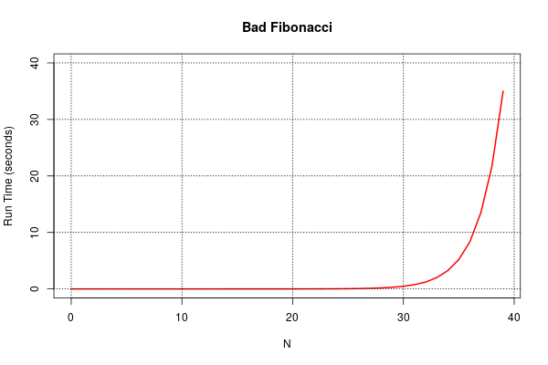
It seems pretty good and then suddenly … It. Just. Crawls.
Reason? The run-time performance T(n) is exponential in n. Specifically
$$ T(n) = \phi^n$$
where \(\phi = \frac{1+\sqrt 5 }{2}\) is the beautiful and magical Golden Ratio.
The fix is easy. The obvious thing to do is when we calculate a Fibonacci number for the first time we store it in a cache. Before we calculate a number we check the cache to see if it has it. That way we stop repeating ourselves. How does this look:
fibcache = {}

def fib2(n):
    """
    A better Fibonacci function.
    :param n: a non-negative integer
    :return: the n'th Fibonacci number
    """
    assert n >= 0
    if n == 0 or n == 1:
        return 1
    if n in fibcache:
        return fibcache[n]
    result = fib2(n - 1) + fib2(n - 2)
    # store the result in the cache!
    fibcache[n] = result
    return result
We use a Python dictionary as our cache.
How does it perform? So much better…
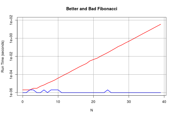
Here we’re using log scales for the Y-axis this time. The red line is the original fib(n) function and the blue line is the new improved fib2(n) function. The blue line is a bit bumpy because I’m not measuring the run-time in a robust way and there is some quantisation effects to boot. I’m not worrying about all that because the lesson is clear in any case.
This clever caching is called memoisation and is a feature of all practical dynamic programming algorithms. It’s the first step towards making recursion smart.
But we aren’t done yet. And this next observation is so so important to practical dynamic programming.
We can eliminate the recursion all together!
Recall the Fibonacci Equation:
$$F_n = F_{n-1} + F_{n-2}$$
Examine the dependencies of \(F_n\).
Notice how the value we want to compute depends ONLY on the previous two values? If we could be certain those values were known then we can eliminate any recursion or caching altogether. We can do this by simply looping – calculating values from low values of \(n\) to high values. This way we only need to remember the previous two values and we don’t need to cache all the values along the way.
Have a look at this sample code:
def fib3(n):
    """
    An even better Fibonacci function.
    :param n: a non-negative integer
    :return: the n'th Fibonacci number
    """
    assert n >= 0
    if n == 0 or n == 1:
        return 1
    b1 = 1
    b2 = 1
    result = 0
    # assert(n > 1)
    for i in range(2, n + 1):
        result = b1 + b2
        # shuffle down
        b1 = b2
        b2 = result
    return result
Before we think about the run time performance I need to make clear in big bright flashing lights – this is what dynamic programming is about. Intelligent recursion. Memoisation and dependency analysis. Analysis which looks at how “simply” reordering the calculations can make the computation efficient. We have considerably cut down the memory storage requirements over the previous example fib2(n) to just two support variables: b1 and b2. Also the run time performance is also clearly \(O(n)\). Sweet!
You might be thinking “You know, that fib3(n) implementation was always the obvious thing to do – nothing special to see here.”
Well I’m pretty sure you won’t be thinking that when we look at some more interesting dynamic programming applications coming up in future planned blogs!
Let’s recap:
- We know about “optimal substructure” and Bellman’s “Principle of Optimality”.
- We know about “memoisation” and intelligent recursion through dependency analysis.
We can now look at some harder problems in dynamic programming.
Oh wait. I mentioned at the beginning that I thought the Fibonacci computation wasn’t a great example of the power of dynamic programming. Why is that, you ask?
Well the answer is: mathematics.
The Fibonacci equation has an explicit closed form solution:
$$ F_n = \frac{\phi_n – \theta_n}{\sqrt 5}$$
where:
- $$\phi = \frac{1+\sqrt 5}{2}$$
- $$\theta = \frac{1-\sqrt 5}{2}$$
The recursive form of the Fibonacci Equation is what mathematicians call linear. And linear equations can be attacked using a whole bunch of additional analysis tools – in this case Z-Transforms. So even though we have fib3(n) running in linear time, we can actually calculate \(F_n\) in constant time – viz \(O(1)\). An exponential improvement over the dynamic programming solution. Very sweet!
The power of dynamic programming is really observed when dealing with nonlinear problems. The Fibonacci numbers don’t demonstrate that. But they do demonstrate the value of mathematics: if you can attack the problem with all the analysis tools you will be ahead. However many real problems are non-linear and non-convex (another tricksy maths term) and dynamic programming can give you real practical solutions if the problem can be shown to have … you guessed it: Optimal Substructure.