This is the second part in a two part post on the Edit Distance algorithm. If you haven’t read the first part yet then you can find it here.

Recap

Remember that Dynamic Programming is a four step process. The last post covered the first two steps of the process for the Edit Distance algorithm. This post covers the last two steps: Memoisation and Iteration Ordering.

Identify the Recursive Structure
Define the States and Actions
Define the Memoisation strategy
Optimise the Iteration Ordering

State and Recursive Formulae

The last post completed the development of the first two steps in the process by writing down the recursive formulation of the edit distance problem as follows:

$ \mathrm{edit}(i,j) = \begin{cases}
i & \text{if } j = 0\\
j & \text{if } i = 0 \\
\min \begin{cases}
\mathrm{edit(i-1,j)} + 1\\
\mathrm{edit(i,j-1)} + 1\\
\mathrm{edit(i-1,j-1)} + \mathbb{I}(X[i] \neq Y[j])
\end{cases} & \text{otherwise}
\end{cases}$

Remember: We defined the following notational convenience for the prefixes of the two strings $X$ and $Y$ whose edit distances we are computing:

$$ \mathrm{edit}(X[1 \ldots i], Y[1 \ldots j]) \equiv \mathrm{edit}(i,j)$$

The length of string $X$ is $M$ units and the length of string $Y$ is $N$ units.

The problem is to calculate $\mathrm{edit}(M,N)$.

Memoisation

Remember: memoisation is simply the idea of caching values of the edit distance function that you have already previously computed – you don’t want to ever recompute the same thing twice!

How many states need to be memoised in this problem?

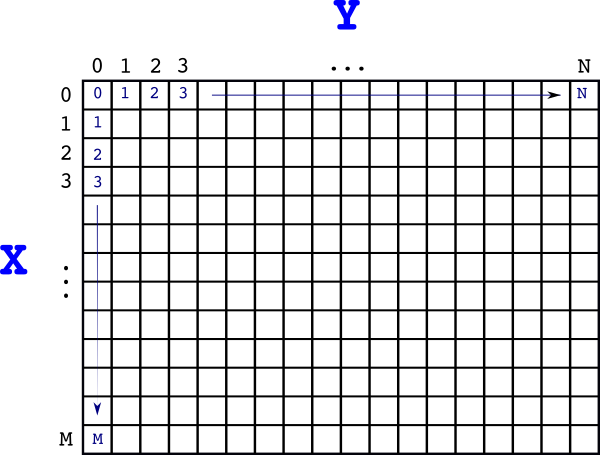
It’s pretty easy to see from the recursive formulae that the states can be enumerated by the tuples $(i,j)$ where $0 \leq i \leq M$ and $0 \leq j \leq N$. Therefore the cache is simply a matrix (two dimensional array) of non-negative integers (edit distances) of size $(M+1) \times (N+1)$ elements.

Let’s call the cache $A$ and denote individual elements as $a_{i,j}$ or $A[i,j]$ depending on context.

We can also initialise it based on the recursive formulae that we developed:

The first row: $i=0 \Rightarrow a_{0,j}=j$
The first column: $j=0 \Rightarrow a_{i,0}=i$

So our matrix $A$ looks like this so far:

Iteration Ordering

The final stage in developing our solution is analysing in what order we should fill out the matrix $A$. This stage is critical to get an efficient algorithm – one that eliminates recursion all together.

As usual, the method for doing this is a dependency analysis of the recursive function that we have developed. For convenience let’s restate the edit distance formulae:

Now, let’s strip this formulae down to its dependencies and let’s also assume that $\mathrm{edit}(i,j) = a_{i,j}$ – that is we’re using our memoised values.

Our dependency relationship looks this:

$ a_{i,j} \leftarrow \begin{cases}
a_{i-1,j}\\
a_{i,j-1}\\
a_{i-1,j-1}
\end{cases}$

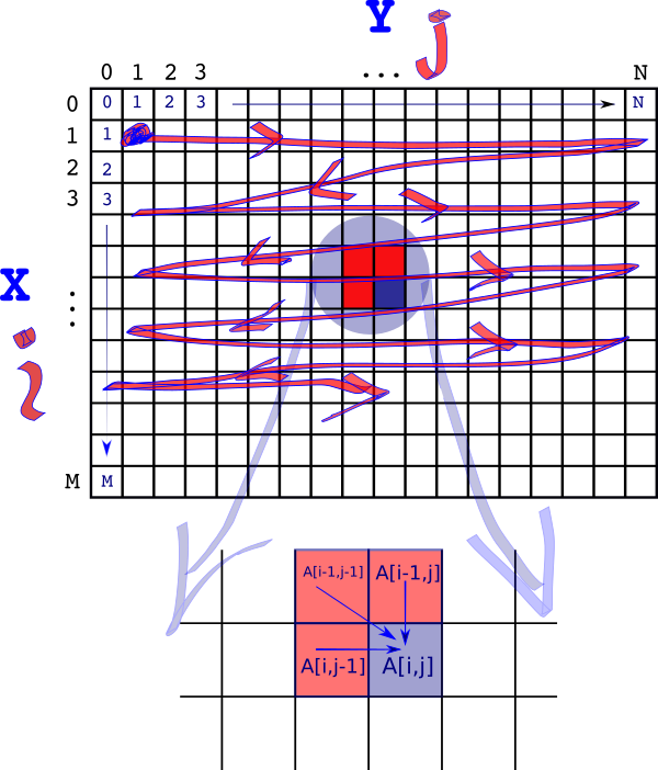
Let’s pick a random element in the cache $A$ – call it $A[i,j]$. The figure below shows it marked in blue. Then the value of $A[i,j]$ depends on the three red squares – $\{A[i-1,j-1], A[i-1, j], A[i,j-1]\}$ representing the three operations $\{Sub/Nop, Insert, Delete\}$ respectively.

Dependency Analysis Determines Iteration Ordering

The goal is to avoid any recursion – the only way we can do that is if the values $A[i,j]$ depends on have already been calculated. This can be achieved if we start our calculation at $A[1,1]$ and then move to $A[1,2],A[1,3]…,A[1,N]$ then $A[2,1],A[2,2],….$ and so on.

So we zig-zag from left to right and top to bottom.

The solution to our problem is then recorded in $A[M,N]$. That is:

$$\mathrm{edit}(M,N) = A[M,N]$$

Implementation

Having got this far the Python implementation is very straightforward.

def edit(s1, s2):
    assert isinstance(s1, str)
    assert isinstance(s2, str)
    rows = len(s1) + 1
    cols = len(s2) + 1
    # Create and initialise the memoisation cache
    distance = [[-1 for col in range(0, cols)] for row in range(0, rows)]    
    # Initialise first row
    for col in range(0, cols):
        distance[0][col] = col  # initialisation
    # Compute the rest of the cache
    for row in range(1, rows):
        for col in range(1, cols):            
            distance[row][0] = row  # initialisation
            # Now compute the non terminal states
            delete = distance[row - 1][col] + 1
            insert = distance[row][col - 1] + 1
            if s1[row - 1] == s2[col - 1]:
                noop = distance[row - 1][col - 1]
                minvalue = min(insert, min(delete, noop))
                distance[row][col] = minvalue                
            else:
                substitute = distance[row - 1][col - 1] + 1
                minvalue = min(insert, min(delete, substitute))
                distance[row][col] = minvalue                
    return distance[rows][cols]

A few things to note:

The matrix $A$ I have called distance in the code.
The variables insert, delete, substitute and noop are the costs of those operations.
My code is not very “pythonic”. I have made the conscious decision to avoid using code idioms that people unfamiliar with Python would find confusing.
The memory requirements are $O(MN)$ – simply the size of the memo-cache.
The run time is also $O(MN)$ – the running time is proportional to the number of elements in the memo-cache that need to be computed.

Let’s look at the memo-cache for our example edit("Thorn","Rose"). This is shown in the table below:

		R	o	s	e
	0	1	2	3	4
T	1	1	2	3	4
h	2	2	2	3	4
o	3	3	2	3	4
r	4	4	3	3	4
n	5	5	4	4	4

The edit distance is simply the value finally computed in the bottom right hand corner – 4!

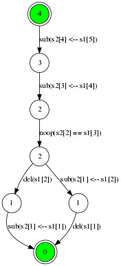
There are two different ways of performing the edit distance. Here is one:

Sub(s2[1] <-- s1[1])
Del(s1[2])
Noop(s2[2] == s1[3])
Sub(s2[3] <-- s1[4])
Sub(s2[4] <-- s1[5])

But what if you want to know how to perform the editing operations and not just the distance?

The editing methods can be reconstructed from the memo-cache. Or built up as part of the main algorithm. Instead of thinking of the memo-cache as a matrix we now think of it as a graphical structure. All the matrix elements now become nodes in the graph. The rules for the graph construction are:

Each matrix element becomes a node.
Edges can be inserted between two nodes in the graph only if
- the matrix elements representing the nodes are adjacent,
- the edge represents either an insert, delete, substitute/noop operation. This restricts the nodes/matrix elements to be the left, above and above-left matrix elements/nodes.
- The edge, whose weight is one, when added satisfies the edit distance formulae.

We now have a graph. Our storage requirements obviously have gone up – we now need memory to store the edges and not just the nodes/matrix elements.

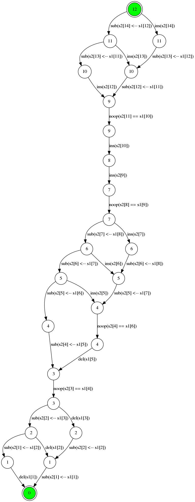
The optimal solutions are all the paths from the “End” node (M,N) in the bottom right hand corner of the memo-cache to the top-left corner “start” node (0,0).

To generate a solution we just walk the graph from end to start and each edge tells us what to do at each step. If a node has more than one outgoing edge we can choose any one – each choice represents a different equally optimal solution.

So for our “Thorn, Rose” example the constructed graph looks like this:

And perhaps a little bit more interesting is the 12 step distance between “Vladimir Putin” and “Donald Trump”:

All the ways of getting from Putin to Trump

Here’s the memo-cache for that:

		V	l	a	d	i	m	i	r		P	u	t	i	n
	0	1	2	3	4	5	6	7	8	9	10	11	12	13	14
D	1	1	2	3	4	5	6	7	8	9	10	11	12	13	14
o	2	2	2	3	4	5	6	7	8	9	10	11	12	13	14
n	3	3	3	3	4	5	6	7	8	9	10	11	12	13	13
a	4	4	4	3	4	5	6	7	8	9	10	11	12	13	14
l	5	5	4	4	4	5	6	7	8	9	10	11	12	13	14
d	6	6	5	5	4	5	6	7	8	9	10	11	12	13	14
	7	7	6	6	5	5	6	7	8	8	9	10	11	12	13
T	8	8	7	7	6	6	6	7	8	9	9	10	11	12	13
r	9	9	8	8	7	7	7	7	7	8	9	10	11	12	13
u	10	10	9	9	8	8	8	8	8	8	9	9	10	11	12
m	11	11	10	10	9	9	8	9	9	9	9	10	10	11	12
p	12	12	11	11	10	10	9	9	10	10	10	10	11	11	12

Wrap Up

So that seems like a lot of work for less than 30 lines of code but I think we got there in the end! I really like this algorithm because it is elegant and it shows how effective dynamic programming is when done properly. And how easy it is to understand when you have the patience to work through it!

There’s lots of applications for the edit distance algorithm. You can imagine applications in bioinformatics, text analysis and even cyber-security. Once you understand the basis of this algorithm it is easy to adapt if for instance the transform operations have different costs or you have completely different transform operations.

At this point, what’s next? I think I want to look at examples where the memo-cache is not an array or matrix but a graph structure. I don’t want people having the impression that all memoisation is array based!