
What we have learned so far about Dynamic Programming are the ideas of “Optimal Substructure” and “Memoisation”. This post will introduce the idea of “Embedding”.
Embedding is the counter-intuitive idea that instead of solving one specific optimisation problem for a value \(N\) you solve all the problems of size less than \(N\) for no extra work.
To look at this idea we’re going to solve the somewhat famous Optimal Money Change Problem.
Imagine you are required to give change for \(N\) dollars. However you can only give change made up of coins made from the following set \(C=\{c_1,c_2,…,c_m\}\).
What is the minimum number of coins you need to make the change?
Most people will just use a greedy approach using largest coins first and then subsequently smaller and smaller coins until the make up the required value. This works well in practice because the values of our coins are designed to give optimal solutions when using the greedy algorithm.
But what is you are using a strange coin system. Let’s be specific. Imagine you can only use coins with the following values:
$$C=\{1,2,7,15,40,99\}$$
and you need to give change for \(N=135\).
Well the Greedy algorithm requires 6 coins to make the change:
Step 1, Value: 135 cents, Give Coin: 99
Step 2, Remaining Value: 36 cents, Give Coin: 15
Step 3, Remaining Value: 21 cents, Give Coin: 15
Step 4, Remaining Value: 6 cents, Give Coin: 2
Step 5, Remaining Value: 4 cents, Give Coin: 2
Step 6, Remaining Value: 2 cents, Give Coin: 2
But the Optimal Solution needs only four coins:
Step 1, Value: 135 cents, Give Coin: 15
Step 2, Remaining Value: 120 cents, Give Coin: 40
Step 3, Remaining Value: 80 cents, Give Coin: 40
Step 4, Remaining Value: 40 cents, Give Coin: 40
Let’s step through solving the problem using the DP methodology:
- Define the state values and actions available for each state.
- Identify the recursive formulation (optimal substructure) that “solves” the problem.
- Design a memoisation scheme that supports the recursion through smart use of memory.
- Analyse the order of iteration with the intent of eliminating recursion altogether.
Step One: State Values and Actions
Define state as the remaining value of change required to be given.
Define the available actions for a state as any coin that could be given as change that doesn’t result in a new state that is negative in value. You can’t give a coin that is larger than the remaining value of change!
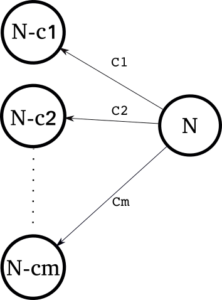
The following diagram is useful. We show for a state N there exists M actions that permit transitions to new smaller states. You might even begin to see how this representation will help with the recursive formulation of the optimum solution… 🙂
Step Two: The Recursive Formulation
The state and actions diagram helps us think about the optimal sub-structure for this problem. We can just right it down:
Let $$s = minchange(N)$$ be the minimum number of coins required for state \(N\).
Therefore we can simply write by inspection of the diagram:
$$ minchange(N) = 1 + \min_{i:N \geq c_i} \{ minchange(N-c_i) \}$$
and obviously \(minchange(0) = 0\).
Maybe the formulae looks a little intimidating at first glance but it simply says that the minimum change required for state \(N\) is simply the minimum number of coins for all the smaller reachable states plus one for using that coin (the action).
Step Three: Memoisation
The memoisation strategy is exactly the same as the Fibonacci memoisation strategy we examined in the previous post: we use a simple linear array indexed by state values \(0 \leq n \leq N\) that stores the value of \(s=minchange(n)\).
Step Four: Iteration Optimisation
Again, exactly like the Fibonacci problem if we iterate from smallest to largest values of the index value we won’t need to use any recursion at all because all the dependencies for calculating state \(n\) will already have been calculated.
Here’s the final code:
def min_change(N, coins):
    """
    Optimum solution for the Minimum Coin Change Problem.
    :param N: The value of change required
    :param coins: a sorted list of coin denominations
    :return: number of coins required
    """
    assert N >= 0
    # assert coins is sorted
    if N == 0:
        return
    # init
    mincoins = {}
    action = {}
    mincoins[0] = 0
    mincoins[1] = 1
    action[0] = 0
    action[1] = 1
    M = len(coins)
    # compute
    for n in range(2, N + 1):
        current = sys.maxint  #
        for i in range(0, M):
            c_i = coins[i]
            if n >= c_i:
                testval = 1 + mincoins[n - c_i]
                if current > testval:
                    # we have a better candidate
                    current = testval
                    mincoins[n] = current
                    action[n] = c_i
            else:
                break  # no need to check larger coins
        # Done for intermediate value n
    # Done! We can emit a solution.
    return mincoins[N]
For comparison here’s the Greedy Solution:
def greedy_change(N, coins):
    """
    Greedy and often non-optimal solution for the Minimum Coin Change Problem.
    :param N: The value of change required
    :param coins: a sorted list of coin denominations
    :return: number of coins required
    """
    assert N >= 0
    # assert coins is sorted
    if N == 0:
        return
    # init
    M = len(coins)
    changecount = 0
    current = N
    idx = M - 1
    # compute
    while current > 0:
        # we iterate from the largest coin to the smallest
        face_value = coins[idx]
        if current >= face_value:
            # we can use this coin
            changecount += 1
            current -= face_value
        else:
            idx -= 1  # use next lowest value coin
    return changecount
Here is an example using the example at the introduction. We want to know how to give change for $$N=135$$ using these very wacky coins: $$C=\{1, 2, 7, 15, 40, 99 \}$$
if __name__ == '__main__':
    value = 135
    face_value_coins = [1, 2, 7, 15, 40, 99]
    face_value_coins.sort()  # must ensure ascending sort order
    # compute solution
    min_change(value, face_value_coins)
    greedy_change(value, face_value_coins)
Final Notes: Embedding
So what is thing called embedding?
Did you notice that when we solved \(minchange(135)\) we also simultaneously and efficiently solved all problems for \(N \le 135\)?
That is embedding.
It seems pretty surprising that to solve a specific problem you solve many other problems at the same time for no apparent extra work. Embedding is characteristic of dynamic programming solutions. It makes sense though because it really is just another way of understanding what “optimal substructure” really means!
In my next post I want to look at a problem that requires a more complex memoisation and optimal iteration strategy. We will start looking at more complex problems 🙂