Dynamic Programming #5 – Edit Distance – Part Two

This is the second part in a two part post on the Edit Distance algorithm. If you haven’t read the first part yet then you can find it here.

Recap

Remember that Dynamic Programming is a four step process. The last post covered the first two steps of the process for the Edit Distance algorithm. This post covers the last two steps: Memoisation and Iteration Ordering.

Identify the Recursive Structure
Define the States and Actions
Define the Memoisation strategy
Optimise the Iteration Ordering

State and Recursive Formulae

The last post completed the development of the first two steps in the process by writing down the recursive formulation of the edit distance problem as follows:

$ \mathrm{edit}(i,j) = \begin{cases}
i & \text{if } j = 0\\
j & \text{if } i = 0 \\
\min \begin{cases}
\mathrm{edit(i-1,j)} + 1\\
\mathrm{edit(i,j-1)} + 1\\
\mathrm{edit(i-1,j-1)} + \mathbb{I}(X[i] \neq Y[j])
\end{cases} & \text{otherwise}
\end{cases}$

Remember: We defined the following notational convenience for the prefixes of the two strings $X$ and $Y$ whose edit distances we are computing:

$$ \mathrm{edit}(X[1 \ldots i], Y[1 \ldots j]) \equiv \mathrm{edit}(i,j)$$

The length of string $X$ is $M$ units and the length of string $Y$ is $N$ units.

The problem is to calculate $\mathrm{edit}(M,N)$.

Memoisation

Remember: memoisation is simply the idea of caching values of the edit distance function that you have already previously computed – you don’t want to ever recompute the same thing twice!

How many states need to be memoised in this problem?

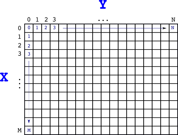
It’s pretty easy to see from the recursive formulae that the states can be enumerated by the tuples $(i,j)$ where $0 \leq i \leq M$ and $0 \leq j \leq N$. Therefore the cache is simply a matrix (two dimensional array) of non-negative integers (edit distances) of size $(M+1) \times (N+1)$ elements.

Let’s call the cache $A$ and denote individual elements as $a_{i,j}$ or $A[i,j]$ depending on context.

We can also initialise it based on the recursive formulae that we developed:

The first row: $i=0 \Rightarrow a_{0,j}=j$
The first column: $j=0 \Rightarrow a_{i,0}=i$

So our matrix $A$ looks like this so far:

Iteration Ordering

The final stage in developing our solution is analysing in what order we should fill out the matrix $A$. This stage is critical to get an efficient algorithm – one that eliminates recursion all together.

As usual, the method for doing this is a dependency analysis of the recursive function that we have developed. For convenience let’s restate the edit distance formulae:

Now, let’s strip this formulae down to its dependencies and let’s also assume that $\mathrm{edit}(i,j) = a_{i,j}$ – that is we’re using our memoised values.

Our dependency relationship looks this:

$ a_{i,j} \leftarrow \begin{cases}
a_{i-1,j}\\
a_{i,j-1}\\
a_{i-1,j-1}
\end{cases}$

Let’s pick a random element in the cache $A$ – call it $A[i,j]$. The figure below shows it marked in blue. Then the value of $A[i,j]$ depends on the three red squares – $\{A[i-1,j-1], A[i-1, j], A[i,j-1]\}$ representing the three operations $\{Sub/Nop, Insert, Delete\}$ respectively.

Dependency Analysis Determines Iteration Ordering

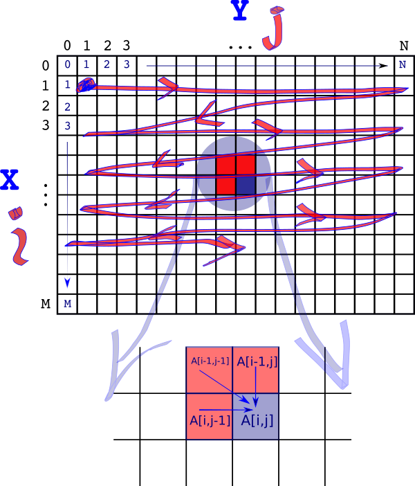
The goal is to avoid any recursion – the only way we can do that is if the values $A[i,j]$ depends on have already been calculated. This can be achieved if we start our calculation at $A[1,1]$ and then move to $A[1,2],A[1,3]…,A[1,N]$ then $A[2,1],A[2,2],….$ and so on.

So we zig-zag from left to right and top to bottom.

The solution to our problem is then recorded in $A[M,N]$. That is:

$$\mathrm{edit}(M,N) = A[M,N]$$

Implementation

Having got this far the Python implementation is very straightforward.

def edit(s1, s2):
    assert isinstance(s1, str)
    assert isinstance(s2, str)
    rows = len(s1) + 1
    cols = len(s2) + 1
    # Create and initialise the memoisation cache
    distance = [[-1 for col in range(0, cols)] for row in range(0, rows)]    
    # Initialise first row
    for col in range(0, cols):
        distance[0][col] = col  # initialisation
    # Compute the rest of the cache
    for row in range(1, rows):
        for col in range(1, cols):            
            distance[row][0] = row  # initialisation
            # Now compute the non terminal states
            delete = distance[row - 1][col] + 1
            insert = distance[row][col - 1] + 1
            if s1[row - 1] == s2[col - 1]:
                noop = distance[row - 1][col - 1]
                minvalue = min(insert, min(delete, noop))
                distance[row][col] = minvalue                
            else:
                substitute = distance[row - 1][col - 1] + 1
                minvalue = min(insert, min(delete, substitute))
                distance[row][col] = minvalue                
    return distance[rows][cols]

A few things to note:

The matrix $A$ I have called distance in the code.
The variables insert, delete, substitute and noop are the costs of those operations.
My code is not very “pythonic”. I have made the conscious decision to avoid using code idioms that people unfamiliar with Python would find confusing.
The memory requirements are $O(MN)$ – simply the size of the memo-cache.
The run time is also $O(MN)$ – the running time is proportional to the number of elements in the memo-cache that need to be computed.

Let’s look at the memo-cache for our example edit("Thorn","Rose"). This is shown in the table below:

		R	o	s	e
	0	1	2	3	4
T	1	1	2	3	4
h	2	2	2	3	4
o	3	3	2	3	4
r	4	4	3	3	4
n	5	5	4	4	4

The edit distance is simply the value finally computed in the bottom right hand corner – 4!

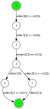
There are two different ways of performing the edit distance. Here is one:

Sub(s2[1] <-- s1[1])
Del(s1[2])
Noop(s2[2] == s1[3])
Sub(s2[3] <-- s1[4])
Sub(s2[4] <-- s1[5])

But what if you want to know how to perform the editing operations and not just the distance?

The editing methods can be reconstructed from the memo-cache. Or built up as part of the main algorithm. Instead of thinking of the memo-cache as a matrix we now think of it as a graphical structure. All the matrix elements now become nodes in the graph. The rules for the graph construction are:

Each matrix element becomes a node.
Edges can be inserted between two nodes in the graph only if
- the matrix elements representing the nodes are adjacent,
- the edge represents either an insert, delete, substitute/noop operation. This restricts the nodes/matrix elements to be the left, above and above-left matrix elements/nodes.
- The edge, whose weight is one, when added satisfies the edit distance formulae.

We now have a graph. Our storage requirements obviously have gone up – we now need memory to store the edges and not just the nodes/matrix elements.

The optimal solutions are all the paths from the “End” node (M,N) in the bottom right hand corner of the memo-cache to the top-left corner “start” node (0,0).

To generate a solution we just walk the graph from end to start and each edge tells us what to do at each step. If a node has more than one outgoing edge we can choose any one – each choice represents a different equally optimal solution.

So for our “Thorn, Rose” example the constructed graph looks like this:

And perhaps a little bit more interesting is the 12 step distance between “Vladimir Putin” and “Donald Trump”:

All the ways of getting from Putin to Trump

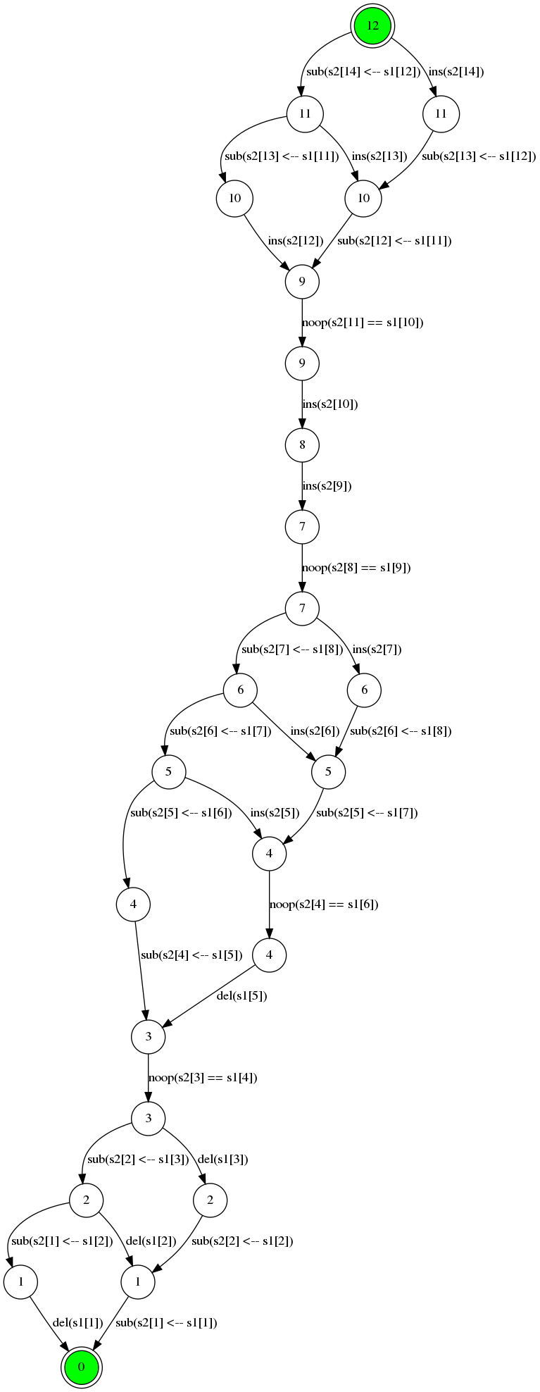
Here’s the memo-cache for that:

		V	l	a	d	i	m	i	r		P	u	t	i	n
	0	1	2	3	4	5	6	7	8	9	10	11	12	13	14
D	1	1	2	3	4	5	6	7	8	9	10	11	12	13	14
o	2	2	2	3	4	5	6	7	8	9	10	11	12	13	14
n	3	3	3	3	4	5	6	7	8	9	10	11	12	13	13
a	4	4	4	3	4	5	6	7	8	9	10	11	12	13	14
l	5	5	4	4	4	5	6	7	8	9	10	11	12	13	14
d	6	6	5	5	4	5	6	7	8	9	10	11	12	13	14
	7	7	6	6	5	5	6	7	8	8	9	10	11	12	13
T	8	8	7	7	6	6	6	7	8	9	9	10	11	12	13
r	9	9	8	8	7	7	7	7	7	8	9	10	11	12	13
u	10	10	9	9	8	8	8	8	8	8	9	9	10	11	12
m	11	11	10	10	9	9	8	9	9	9	9	10	10	11	12
p	12	12	11	11	10	10	9	9	10	10	10	10	11	11	12

Wrap Up

So that seems like a lot of work for less than 30 lines of code but I think we got there in the end! I really like this algorithm because it is elegant and it shows how effective dynamic programming is when done properly. And how easy it is to understand when you have the patience to work through it!

There’s lots of applications for the edit distance algorithm. You can imagine applications in bioinformatics, text analysis and even cyber-security. Once you understand the basis of this algorithm it is easy to adapt if for instance the transform operations have different costs or you have completely different transform operations.

At this point, what’s next? I think I want to look at examples where the memo-cache is not an array or matrix but a graph structure. I don’t want people having the impression that all memoisation is array based!

December 4, 2017May 31, 2021

Dynamic Programming #4 – Edit Distance – Part One

So just how close is s1 = "Vladimir Putin" and s2 = "Donald Trump" really?

My claim is that the distance between them is 12 steps.

What am I talking about?

This post is all about the edit distance between two strings. The edit distance is the minimum number of transformation operations that can turn one string into the other. The edit distance is also called the Levenshtein Distance named after Vladimir Levenshtein who sadly died just a few months ago.

As you can imagine there are many types of transformations you can do to a string but in the edit distance case there are three specific operations that can be applied to single character positions – let’s say at position i in the string:

Insert a character
Delete a character
Substitute a character

So we have three actions at each position we can perform. We also assume that each operation costs exactly the same (one unit) – but it’s easy to change this depending on the specific problem being considered.

My first three posts on dynamic programming have laid out all the basics we need to work out how to compute the edit distance between two strings efficiently. I strongly recommend reading them first because we will be using all the machinery to get to our algorithm! After this post, I’m hoping you will come away with a good appreciation of the real power of applied dynamic programming too.

Let’s recall the four step Dynamic Programming process:

Identify the recursive structure (“optimal substructure”)
Define the States and Actions
Define the memoisation strategy
Optimise the iteration ordering

Steps one and two are the hard ones. And there is usually some trial and error before getting that flowing. Steps three and four are much easier but are the key to getting the algorithm performing efficiently.

Recursive Structure

I think the best way to explain the process is with a small example. Let’s say we want to find the distance between two strings:

s1 = "THORN" and
s2 = "ROSE"

These two strings are small enough that we can see that if we align the two strings at the letter “O” then by inspection we can see the edit distance is 4. The third row gives an operation to perform at each position – note: “Nop” is a no-operation –
a virtual operation that means don’t do anything. The fourth row is the cost of each operation – so the row sum gives the edit distance.

s1:	T	H	O	R	N
s2:	R		O	S	E
Op:	Sub	Del	Nop	Sub	Sub
Cost:	1	1	0	1	1

How does this help?

Let’s assume this table is an optimal representation of edit transformations (it is). Consider the prefix (first four columns) and the last column separately. The cost of the optimal transformation between “THORN” and “R*OSE” is the cost of optimal transformations between “THOR” and “R*OS” plus one.

Note: the “*” is just a placeholder for the fact that the two strings are different lengths and some alignment needs to occur.

Like many string algorithms the recursive formulation separates the prefix from the suffix – which in our case is the last column. If you’re a bit lost stick with it – it will be come clearer after you get through the next section.

States and Actions

We’ve already mentioned our set of action operations:

$$A=\{Ins,Del,Sub,Nop\}$$

The State definition is more interesting. The key observation in the previous section is that we separate prefixes of both strings in the recursive formulation. Let’s call both strings $X$ and $Y$. So $X[1..i]$ denotes the prefix of $X$ consisting of the first $i$ characters. Similarly, $Y[1..j]$ is the prefix of $Y$ containing the first $j$ characters.

So state consists of a tuple of the two prefixes:

$$\mathrm{state}: (X[1\ldots i],Y[1\ldots j])$$

Let’s define the length of $X$ to be $M$ characters long. Similarly, the length of $Y$ is $N$ characters.

Let’s give our optimal edit distance function the following signature:

$\mathrm{edit}(X[1\ldots M],Y[1\ldots N]) \mapsto \mathbb{N}$

Remember: When we are developing our dynamic programming algorithms they are a mapping from state to value. We need to do this to capture and express mathematically the recursive formulation (“optimal substructure”) in the problem. Also, it allows us to think in terms of a graphical model of the problem: two states (“vertices”) are connected (“edge”) if a single action/operation performed at one state transform it into the second state. You will see this explicitly later.

Finally, let’s denote the null/empty string as $\emptyset$.

Write It Down

It’s a bit of work but we’re getting there. We want to write down mathematically a recurrence formulae for the edit distance:

First, assume $X$ and $Y$ are not null.

Given a specific state $(X[1\ldots i],Y[1\ldots j]) $, there are three possibilities we need to consider:

$X$ is longer than $Y$:
Action: insert a character
$X$ is shorter than $Y$:
Action: delete a character
$X$ is the same length as $Y$:
Action: either substitute a character or it’s a no-operation.

Each of these possibilities have three different recurrence formulaes for the edit distance:

Insert: $\mathrm{edit}(X[1\ldots M],Y[1\ldots N]) = 1 +\mathrm{edit}(X[1 \ldots M-1],Y[1\ldots N]) $
Delete: $\mathrm{edit}(X[1\ldots M],Y[1 \ldots N]) = 1 +\mathrm{edit}(X[1\ldots M],Y[1\ldots N-1]) $
Substitute or Nop: $\mathrm{edit}(X[1\ldots M],Y[1\ldots N]) = \mathbb{I}(X[M] \neq Y[N]) +\mathrm{edit}(X[1\ldots M-1],Y[1\ldots N-1]) $

Note: $\mathbb{I}$ is the indicator function – it equals one if the predicate inside is True and zero if the predicate is False. Here it simply tests if a character substitution is required and adds a unit cost if so.

We can now define the edit distance as the following recursion:

$ \mathrm{edit}(X[1\ldots M],Y[1\ldots N]) = \min \begin{cases}
1 + \mathrm{edit}(X[1 \ldots M-1],Y[1\ldots N])\\
1 + \mathrm{edit}(X[1\ldots M],Y[1\ldots N-1])\\
\mathbb{I}(X[M] \neq Y[N]) + \mathrm{edit}(X[1\ldots M-1],Y[1\ldots N-1])
\end{cases} $

Base Cases

So how do we stop recursing?

There are three separate stopping conditions:

$X \equiv \emptyset $
Action: Insert $N$ characters to make $Y$
$Y \equiv \emptyset $
Action: Insert $M$ characters to make $X$
$X \equiv \emptyset \mathrm \, {and} \, Y \equiv \emptyset$
Action: Define the distance to be zero.

Ok… it’s getting tedious writing out all the indexations for the all strings. Because we are dealing with prefixes let’s just agree to the following convention: it will make our code and maths look simpler!

Define: $$ \mathrm{edit}(X[1 \ldots i], Y[1 \ldots j]) \equiv \mathrm{edit}(i,j)$$

So our recursion with the base cases included looks like this:

Having got this far I reckon it’s a good place to pause because it’s getting quite long for a single blog post – and then continue in “Edit Distance – Part Two”. We will obviously look at the next two steps in the Dynamic Programming methodology – Memoisation and Iteration Ordering. And of course – some Python code and examples!

November 14, 2017May 31, 2021

Dynamic Programming – An Introduction #3

What we have learned so far about Dynamic Programming are the ideas of “Optimal Substructure” and “Memoisation”. This post will introduce the idea of “Embedding”.

Embedding is the counter-intuitive idea that instead of solving one specific optimisation problem for a value $N$ you solve all the problems of size less than $N$ for no extra work.

To look at this idea we’re going to solve the somewhat famous Optimal Money Change Problem.

Imagine you are required to give change for $N$ dollars. However you can only give change made up of coins made from the following set $C=\{c_1,c_2,…,c_m\}$.

What is the minimum number of coins you need to make the change?

Most people will just use a greedy approach using largest coins first and then subsequently smaller and smaller coins until the make up the required value. This works well in practice because the values of our coins are designed to give optimal solutions when using the greedy algorithm.

But what is you are using a strange coin system. Let’s be specific. Imagine you can only use coins with the following values:

$$C=\{1,2,7,15,40,99\}$$

and you need to give change for $N=135$.

Well the Greedy algorithm requires 6 coins to make the change:

Step 1, Value: 135 cents, Give Coin: 99
Step 2, Remaining Value: 36 cents, Give Coin: 15
Step 3, Remaining Value: 21 cents, Give Coin: 15
Step 4, Remaining Value: 6 cents, Give Coin: 2
Step 5, Remaining Value: 4 cents, Give Coin: 2
Step 6, Remaining Value: 2 cents, Give Coin: 2

But the Optimal Solution needs only four coins:

Step 1, Value: 135 cents, Give Coin: 15
Step 2, Remaining Value: 120 cents, Give Coin: 40
Step 3, Remaining Value: 80 cents, Give Coin: 40
Step 4, Remaining Value: 40 cents, Give Coin: 40

Let’s step through solving the problem using the DP methodology:

Define the state values and actions available for each state.
Identify the recursive formulation (optimal substructure) that “solves” the problem.
Design a memoisation scheme that supports the recursion through smart use of memory.
Analyse the order of iteration with the intent of eliminating recursion altogether.

Step One: State Values and Actions

Define state as the remaining value of change required to be given.

Define the available actions for a state as any coin that could be given as change that doesn’t result in a new state that is negative in value. You can’t give a coin that is larger than the remaining value of change!

The following diagram is useful. We show for a state N there exists M actions that permit transitions to new smaller states. You might even begin to see how this representation will help with the recursive formulation of the optimum solution… 🙂

Step Two: The Recursive Formulation

The state and actions diagram helps us think about the optimal sub-structure for this problem. We can just right it down:

Let $$s = minchange(N)$$ be the minimum number of coins required for state $N$.

Therefore we can simply write by inspection of the diagram:

$$ minchange(N) = 1 + \min_{i:N \geq c_i} \{ minchange(N-c_i) \}$$

and obviously $minchange(0) = 0$.

Maybe the formulae looks a little intimidating at first glance but it simply says that the minimum change required for state $N$ is simply the minimum number of coins for all the smaller reachable states plus one for using that coin (the action).

Step Three: Memoisation

The memoisation strategy is exactly the same as the Fibonacci memoisation strategy we examined in the previous post: we use a simple linear array indexed by state values $0 \leq n \leq N$ that stores the value of $s=minchange(n)$.

Step Four: Iteration Optimisation

Again, exactly like the Fibonacci problem if we iterate from smallest to largest values of the index value we won’t need to use any recursion at all because all the dependencies for calculating state $n$ will already have been calculated.

Here’s the final code:

def min_change(N, coins):
    """
    Optimum solution for the Minimum Coin Change Problem.    
    :param N: The value of change required
    :param coins: a sorted list of coin denominations
    :return: number of coins required
    """
    assert N >= 0
    # assert coins is sorted
    if N == 0:
        return
    # init
    mincoins = {}
    action = {}
    mincoins[0] = 0
    mincoins[1] = 1
    action[0] = 0
    action[1] = 1
    M = len(coins)
    # compute
    for n in range(2, N + 1):
        current = sys.maxint  #
        for i in range(0, M):
            c_i = coins[i]
            if n >= c_i:
                testval = 1 + mincoins[n - c_i]
                if current > testval:
                    # we have a better candidate
                    current = testval
                    mincoins[n] = current
                    action[n] = c_i
            else:
                break  # no need to check larger coins
        # Done for intermediate value n        
    # Done! We can emit a solution.
    return mincoins[N]

For comparison here’s the Greedy Solution:

def greedy_change(N, coins):
    """
    Greedy and often non-optimal solution for the Minimum Coin Change Problem.
    :param N: The value of change required
    :param coins: a sorted list of coin denominations
    :return: number of coins required
    """
    assert N >= 0
    # assert coins is sorted
    if N == 0:
        return
    # init
    M = len(coins)
    changecount = 0
    current = N
    idx = M - 1
    # compute
    while current > 0:
        # we iterate from the largest coin to the smallest
        face_value = coins[idx]
        if current >= face_value:
            # we can use this coin
            changecount += 1            
            current -= face_value
        else:
            idx -= 1  # use next lowest value coin
    return changecount

Here is an example using the example at the introduction. We want to know how to give change for $$N=135$$ using these very wacky coins: $$C=\{1, 2, 7, 15, 40, 99 \}$$

if __name__ == '__main__':
    value = 135
    face_value_coins = [1, 2, 7, 15, 40, 99]   
    face_value_coins.sort()  # must ensure ascending sort order 
    # compute solution
    min_change(value, face_value_coins)
    greedy_change(value, face_value_coins)

Final Notes: Embedding

So what is thing called embedding?

Did you notice that when we solved $minchange(135)$ we also simultaneously and efficiently solved all problems for $N \le 135$?

That is embedding.

It seems pretty surprising that to solve a specific problem you solve many other problems at the same time for no apparent extra work. Embedding is characteristic of dynamic programming solutions. It makes sense though because it really is just another way of understanding what “optimal substructure” really means!

In my next post I want to look at a problem that requires a more complex memoisation and optimal iteration strategy. We will start looking at more complex problems 🙂

October 21, 2017May 31, 2021

Dynamic Programming – An Introduction #2

The last post talked about Bellman’s Principle of Optimality. This is the idea that some problems have “optimal substructure” which allows for an equation to be written down which is a recursive expression of the problem. This recursive equation is called the Bellman Equation of the problem.

This post is about memoisation – a technique that makes the computation of those nasty recursion equations more tractable in practice.

The traditional approach to explaining memoisation is to use the calculation of Fibonacci numbers as a demonstration. The Fibonacci numbers are calculated from a beautifully simple recurrence equation

$$F_n = F_{n-1} + F_{n-2}$$

where the first two numbers in the series are defined as 0 and 1.

I hadn’t wanted to do that because I wanted to be a little fresh in my approach. More importantly the Fibonacci series is not a good example of the power of dynamic programming. Why? Read on.

So, we are going to solve the Fibonacci computation using dynamic programming. Then we’re going to look at why it’s not a great example of the technique. The reasons are important and interesting.

First the naive computation of the Fibonacci numbers directly implements the recurrence relation as follows:

def fib(n):
    """
    Bad Fibonacci function.
    :param n: a non-negative integer
    :return: the n'th Fibonacci number
    """
    assert n >= 0
    if n == 0 or n == 1:
        return 1
    result = fib(n - 1) + fib(n - 2)
    return result

Why is this so bad?

It’s terribly slow. Let’s look at fib(5):

 fib(5) = fib(4) + fib(3)

but

fib(4) = fib(3) + fib(2)

fib(3) = fib(2) + fib(1)

fib(2) = fib(1) + fib(0)

fib(1) = 1

fib(0) = 1

Can you see what’s going on? We keep calculating the same numbers over and over again.

How bad can it be in practice? Terrible: Look at these plot:

It seems pretty good and then suddenly … It. Just. Crawls.

Reason? The run-time performance T(n) is exponential in n. Specifically

$$ T(n) = \phi^n$$

where $\phi = \frac{1+\sqrt 5 }{2}$ is the beautiful and magical Golden Ratio.

The fix is easy. The obvious thing to do is when we calculate a Fibonacci number for the first time we store it in a cache. Before we calculate a number we check the cache to see if it has it. That way we stop repeating ourselves. How does this look:

fibcache = {}

def fib2(n):
    """
    A better Fibonacci function.
    :param n: a non-negative integer
    :return: the n'th Fibonacci number
    """
    assert n >= 0
    if n == 0 or n == 1:
        return 1
    if n in fibcache:
        return fibcache[n]
    result = fib2(n - 1) + fib2(n - 2)
    # store the result in the cache!
    fibcache[n] = result
    return result

We use a Python dictionary as our cache.

How does it perform? So much better…

Here we’re using log scales for the Y-axis this time. The red line is the original fib(n) function and the blue line is the new improved fib2(n) function. The blue line is a bit bumpy because I’m not measuring the run-time in a robust way and there is some quantisation effects to boot. I’m not worrying about all that because the lesson is clear in any case.

This clever caching is called memoisation and is a feature of all practical dynamic programming algorithms. It’s the first step towards making recursion smart.

But we aren’t done yet. And this next observation is so so important to practical dynamic programming.

We can eliminate the recursion all together!

Recall the Fibonacci Equation:

$$F_n = F_{n-1} + F_{n-2}$$

Examine the dependencies of $F_n$.

Notice how the value we want to compute depends ONLY on the previous two values? If we could be certain those values were known then we can eliminate any recursion or caching altogether. We can do this by simply looping – calculating values from low values of $n$ to high values. This way we only need to remember the previous two values and we don’t need to cache all the values along the way.

Have a look at this sample code:

def fib3(n):
    """
    An even better Fibonacci function.
    :param n: a non-negative integer
    :return: the n'th Fibonacci number
    """
    assert n >= 0
    if n == 0 or n == 1:
        return 1
    b1 = 1
    b2 = 1
    result = 0
    # assert(n > 1)
    for i in range(2, n + 1):
        result = b1 + b2
        # shuffle down
        b1 = b2
        b2 = result
    return result

Before we think about the run time performance I need to make clear in big bright flashing lights – this is what dynamic programming is about. Intelligent recursion. Memoisation and dependency analysis. Analysis which looks at how “simply” reordering the calculations can make the computation efficient. We have considerably cut down the memory storage requirements over the previous example fib2(n) to just two support variables: b1 and b2. Also the run time performance is also clearly $O(n)$. Sweet!

You might be thinking “You know, that fib3(n) implementation was always the obvious thing to do – nothing special to see here.”
Well I’m pretty sure you won’t be thinking that when we look at some more interesting dynamic programming applications coming up in future planned blogs!

Let’s recap:

We know about “optimal substructure” and Bellman’s “Principle of Optimality”.
We know about “memoisation” and intelligent recursion through dependency analysis.

We can now look at some harder problems in dynamic programming.

Oh wait. I mentioned at the beginning that I thought the Fibonacci computation wasn’t a great example of the power of dynamic programming. Why is that, you ask?

Well the answer is: mathematics.

The Fibonacci equation has an explicit closed form solution:

$$ F_n = \frac{\phi_n – \theta_n}{\sqrt 5}$$

where:

$$\phi = \frac{1+\sqrt 5}{2}$$
$$\theta = \frac{1-\sqrt 5}{2}$$

The recursive form of the Fibonacci Equation is what mathematicians call linear. And linear equations can be attacked using a whole bunch of additional analysis tools – in this case Z-Transforms. So even though we have fib3(n) running in linear time, we can actually calculate $F_n$ in constant time – viz $O(1)$. An exponential improvement over the dynamic programming solution. Very sweet!

The power of dynamic programming is really observed when dealing with nonlinear problems. The Fibonacci numbers don’t demonstrate that. But they do demonstrate the value of mathematics: if you can attack the problem with all the analysis tools you will be ahead. However many real problems are non-linear and non-convex (another tricksy maths term) and dynamic programming can give you real practical solutions if the problem can be shown to have … you guessed it: Optimal Substructure.

October 12, 2017May 31, 2021

Dynamic Programming – An Introduction #1

Dynamic programming is a super power.

Once you understand what it is, how it works and grasp the many applications it has in both computing and in mathematical optimisation you will feel … special.

Maybe even … elite.

First a bit of history.

Richard Bellman published a very influential set of books and papers in the 1950s and 60s using the technique he named “Dynamic Programming”. Despite the weird name his technique was able to solve some very complex problems in operations research – which is the name for applied mathematics in problems that people in industry, government and defence care about.

DP is based on Bellman’s Principle of Optimality:

An optimal policy has the property that whatever the initial state and initial decision are, the remaining decisions must constitute an optimal policy with regard to the state resulting from the first decision.

Imagine you are in the town of START which has two roads to the town of END – the High road and the Low road. Now 50 km down the High road is the town of A and 20 km down the Low road is the town of B. Furthermore someone clever has already worked out the shortest path from A to End and B to End which have many towns along the way – perhaps the paths even overlap. Have look at the figure:

Bellman’s optimality principle means in practice that the shortest path from Start to End is the minimum of :

High Road: $$Distance(Start, End)_A =dist(A) + Distance(A, End)$$ or 380 km.
Low Road: $$Distance(Start, End)_B = dist(B) + Distance(B, End)$$ or 410 km.

Bellman Equation: $$Distance(Start,End) = \min_i \{ d_{start,i} + Distance(i, End) $$

The proof is almost by definition. Assume there was a shorter path. Then we get an immediate contradiction: we asserted a priori that we knew the shortest paths from A and B to End. If there exists a shorter path then someone is lying.

I can’t decide if Bellman’s principle is profound or just obvious. Both I guess. But it is an enormous enabler because it allows us to write down a recursive equation for our optimisation problem known as the Bellman Equation. Solving the Bellman equation for a problem may be very difficult in practice but it is the starting point for analysing the problem in depth.

Dynamic Programming problems generally have these kind of features:

“Optimal Substructure”: The solution to the problem can be modelled recursively using solutions to smaller problems. This is the same idea as Bellman’s Optimality Principle and his equation. I also want to say that this is NOT the same thing as “divide and conquer” which relies on solving disjoint sub-problems independently.
Solutions generally involve a sequence of decision operations with each decision depending on the state at that time.
Often you can represent the problem as a graphical model in which you are looking for either the longest or shortest path from beginning to end.

All we have done so far is just give an introduction the main ideas of DP and some of the language involved. So far you won’t have noticed any glowing new super powers but we are on the high road towards dynamic programming enlightenment.

Next I want to show a very simple example of practical DP. From there I will build up to some more complex problems.

It Must Be Beautiful

Posts